Let's look at the Xpander filter a little more closely. The structure is similar to the generic 4 pole filter. If you haven't gone through that, it should be considered a requisite. If you set the A term from the base 4 pole filter to 0, the two are structurally equivalent, although here we're using A as the amplification factor starting on V₁. Additionally, in the Xpander 3 pole modes the first filter pole has its pole moved upwards by a factor of 330. We've included that pole in the calculations.

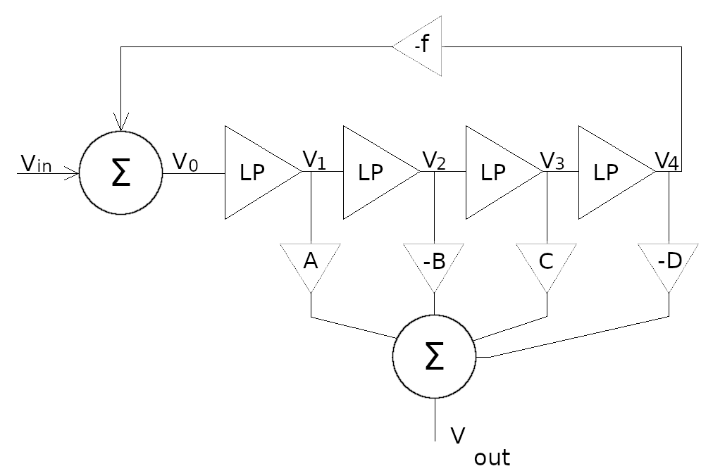
1. Solving for V₀ to V₄

   V0	= Vin - fV4
   V1	= V0(.0030303s+1)	Here, we're adding a factor to account for the way the Xpander switches out it's first low pass stage, by simply moving the pole to a very high frequency. The ratio of the capacitor values is 33nF:.1nF or 330:1.
   V2	= V1(s+1)	= V0(.0030303s + 1)(s+1)
   V3	= V2(s+1)	= V0(.0030303s + 1)(s+1)^2
   V4	= V3(s+1)	= V0(.0030303s + 1)(s+1)^3

   Therefore
   

   V4	= Vin - fV4(.0030303s + 1)(s+1)^3
   Let's define Den3 = (.0030303s + 1)(s+1)^3
   V4	= Vin - fV4Den3
   V4Den3	= Vin - fV4
   V4Den3 + fV4	= Vin
   V4(Den3 + f)	= Vin
   V4Vin	= 1(Den3 + f)
   So we have the transfer function for V4. Now, it's helpful to divide the top and bottom by Den3.	=  1 Den3 1 Den3 (Den3 + f)
   	=  1 Den3 1 + f Den3
   	=  1 Den3 (1 + f Den3 )
   This is a convenient form as it lets us rewrite the V4 transfer function in a form that looks like the standard 4 pole LP transfer function with an added F term. The original form with small f will be used later when expanding the common denominator	1 Den3 F where F = 1 + fDen3

   
   With the transfer function in this form, we can easily define V₁, V₂, and V₃ by adding succesive (s+1) terms to the numerator and reducing. We don't have a need for V₀:
   V₄ = 1Den₃ F = 1(.0030303s + 1)(s+1)^3 FV_in
   V₃ = (s+1)Den₃ F = 1(.0030303s + 1)(s+1)^2 FV_in
   V₂ = (s+1)^2Den₃ F = 1(.0030303s + 1)(s+1) FV_in
   V₁ = (s+1)^3Den₃ F = 1(.0030303s + 1) FV_in
   
   

   Now we can sum the individual responses into our mixing network.

2. Mix equation for 4 poles with feedback

   We can see that V_out is just AV₁ - BV₂ + CV₃ - DV₄
   Substituting the transfer functions we found previously gives us:
   V_outV_in = A(.0030303s + 1) F - B(.0030303s + 1)(s+1) F + C(.0030303s + 1)(s+1)^2 F - D(.0030303s + 1)(s+1)^3 F
   
   the common denominator is (.0030303s + 1)(s+1)^3 F, so we can multiply each by the common denominator, cancel the common terms and expand the (s+1) exponential terms. Note that all of the F terms will cancel.

3. Numerators

   A(s+1)^3	=>	As^3	3As^2	3As	+ A
   -B(s+1)^2	=>		-Bs^2	- 2Bs	- B
   C(s+1)	=>			Cs	+ C
   D	=>				- D
   		+ As^3	+ (3A - B)s^2	+ (3A - 2B + C)s	A - B + C - D

   
   
   As it turns out, this is the same numerator polynomial you get with or without feedback, due to the cancellations of the F terms. The F term will only appear in the denominator. We also don't end up with the shifted pole term (.0030303s + 1) in the numerator since we're not using V₀.

4. Combined numerator coefficients

   replacing s with jw, we can group the real and imaginary parts
   
   real terms: R = -(3A - B)w^2 + (A - B + C - D)
   imaginary terms: I = j [ -Aw^3 + (3A - 2B + C)w ]
   
   The magnitude of the numerator can then be found by Mag_n = √( R^2 + I^2 )

5. Denominator

   The common denominator is Den₃F. We showed before that
   Den₃ F = Den₃ + f    (note big F on left and small f on right)
   
   

   Den3 + f	= (.0030303s + 1)(s+1)^3 + f
   	= (.0030303s + 1)(s^3 + 3s^2 + 3s + 1) + f
   	= (.0030303s^4 + 1.0090909s^3 + 3.0090909s^2 + 3.0030303s + 1 + f

   real terms: R = .0030303w^4 - 3.0090909w^2 + 1 + f
   imaginary terms: I = j [ -1.0090909w^3 + 3.0030303w ]
   
   The magnitude of the denominator can likewise be found by Mag_d = √( R^2 + I^2 )
6. The total magnitude is then just Mag_n / Mag_d

References and further reading

• Electric Druid has more discussion of the Xpander / Matrix 12 modes, as well as schematics of a modern take on pole mixing and links to even more reading.